To help stay competitive and maximize employee productivity, organizations should continually ensure that their teams are up to speed with the latest Excel functionalities and are routinely seeking to enhance efficiency in Excel analyses. Spreadsheet software was introduced with VisiCalc back in 1979, and has dramatically progressed to the Office 365 Excel today! Many employees get comfortable with the spreadsheet versions they learned on, and as more options become available to accomplish the same task in different manners, there is a tendency to get stuck in the old ways. Maybe there are a few new capabilities in each upgrade that are capitalized on, but unless a conscientious decision is made to start using a particular new function, employees often lose sight of the various new tools.
Excel developers understand old habits are hard to break and help by maintaining ways to use commands in the old familiar way. As an example, for those who get frustrated finding the function desired on the correct ribbon, Excel has added the Quick Access Toolbar to the top of the worksheet which can be customized for frequently used routine commands.

Spreadsheets are best set up when the data is in a database format (a header row that includes labels in each column, followed by data below the header row). This permits easy use of filters, sorting, pivots, etc. Establishing ‘Tables’ for your database can be beneficial as they automatically include various filter and sorting options with the dropdown arrows in each column. Tables also permit automatic extension of rows and columns as additional data is added. (To create a Table, highlight all database cells and use CTRL-T). This invokes the Table Tools menu with options for table styles. It allows Name Ranges for column headings to be established for easy reference by formulas (with cursor in table, click on the Formulas menu and select ‘Create from Selection’). In Formulas, Table Names are shown in (parentheses) and Name Ranges are shown in [brackets]. For Filters, one capability not readily known to many users, is the ‘add current selection to filter’ option. This is available when a filter is applied and another item needs to be added to the filter.
The CTRL and ALT Keys permit quick activations of various functions. A few examples include, ‘CTRL-Z’ for undo; ‘CTRL-SHFT-1’ to apply the comma format; ‘ALT=’ for =SUM(); and ‘ALT-N-V’ to create a Pivot Table. Don’t forget to use the ‘Select Current Range’ Icon (in your Quick Access Toolbar, if saved to this toolbar) to highlight the database prior to clicking ‘ALT-N-V’. 
The =TRIM function is a handy tool as it eliminates leading spaces, trailing spaces, reduces spaces between words to one, and removes formats inherent in the digits in a cell. This is often useful for data downloaded from systems, particularly when applying the =vlookup formula, (which require matching exact formats). As you start to enter a formula, and you see the formula desired, hit ‘Tab’ to accept the formula (without the need to type the entire formula).
Those familiar with the =vlookup function understand its limitation of requiring the matching data to be in the far-left column (first column) of the array. This often requires moving data around or adding additional columns of duplicated data so the column is in the correct position.
Excel has two functions that can be used together to help eliminate this issue, but they tend to be complex. One is the Match function, which simply indicates the position of a match (i.e. a result of 9 means it is in the 9th row); the other is the INDEX function which permits pulling data out of a list based on a row reference and column reference. The Index and Match functions used together work similar to a vlookup, but are designed for when you need a left lookup
Excel recently released the =xlookup function (similar to a vlookup, but without restrictions of positioning columns and simpler to use than the Index/Match functions. In the example below, cell G2 would have ‘=xlookup(F2,B:B,D:D)’ where F2 is the lookup value to be matched in column B; if there is a match, it returns the corresponding row data that is shown in column D. You can also add ,”None” to the end of the formula before the closed parenthesis so Excel will show ‘None’ on matches that do not exist.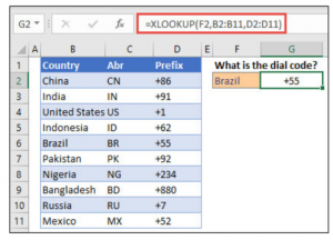
A few other fun Office 365 features worth exploring. Dragging a column of formulas right or left using the right mouse allows you to copy back in place as values, removing the formulas.
Pivot tables now have the option to insert filter slicers. 
Filter slicers allow you to hone in on the specific data you need within the pivot table (with your mouse in a cell in the pivot table, click on insert Filters Slicer). Excel has also added Comment threads to permit others to add to your comments in cells (the old comment option has been replaced and now is shown as Notes). Don’t forget to check out the Insert Icons as well, to visually communicate using symbols.
With so many changes to Excel, it’s important to continue to become familiar with new features and assess their usefulness for you. You-tube videos are wonderful with showing how commands work. LinkedIn Learning has some fabulous courses as well. Also, in the middle top of the Excel workbook is an area with a light-bulb icon that says ‘Tell me what you want to do’ and is great for quick searches. Remember… Explore and attempt! The more familiar your team is with Excel functionality; the faster they can assist in achieving the organizational goals.
CHECK OUT OUR STREAMLINING & AUTOMATION WEBINAR WITH FEI on this subject.
Ilene Kappel, Director – Sirius Solutions, L.L.L.P.
If you would like further information regarding Streamlining and Automation, please complete the form below.
[contact-form-7 id=”227245″ title=”Contact Us”]